Hopf Fibration of 3-sphere
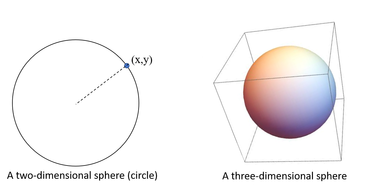
Our world consists of 3 spatial dimensions and 1 time dimension. But how to perceive or visualize 4 spatial dimensions? Well, there are a number of ways to do so. There are several good examples here and there of visualizing the 4 dimensions using a hypercube (A cube that lives in 4-dimensional space). Here we are going to discuss another way of visualizing the 4-dimensional world by dissecting a sphere that lives in 4 spatial dimensions, a 3-sphere.Hopf Fibration T-Shirt
Show off your love for advanced mathematics with this stylish Hopf fibration t-shirt. Perfect for anyone who appreciates the elegance of higher-dimensional geometry.
- High-quality print of the Hopf fibration
- Available in various sizes
- 100% cotton for comfort
- Great conversation starter!
 Now, hold your breath, we are going to progress to the next level, a three-sphere. The three-sphere is a sphere that resides in the 4-dimensional space and it fulfills these conditions:
\begin{equation}
x_1^2+x_2^2+x_3^2+x_4^2=r
\end{equation}
where $x_1,...x_4$ are the four spatial coordinate axes. Therefore, a 4-sphere is hard to imagine since the world that we are living in consists of only 3 spatial dimensions.
The Hopf fibration is a projection map from the three-sphere to the two-sphere. It shows how the three-sphere can be built by a collection of circles arranged like points on a two-sphere. An example of the visualization of Hopf Fibration is by using the stereographic projection from the "south pole" of $S^3$ onto an equatorial hyperplane $R^3$
To begin with, we express the complex coordinates of single qubit into their respective real and imaginary parts:
\begin{equation}
Z_0=u+v\textbf{i} , Z_1 = u'+v'\textbf{j}
\end{equation}
Now, hold your breath, we are going to progress to the next level, a three-sphere. The three-sphere is a sphere that resides in the 4-dimensional space and it fulfills these conditions:
\begin{equation}
x_1^2+x_2^2+x_3^2+x_4^2=r
\end{equation}
where $x_1,...x_4$ are the four spatial coordinate axes. Therefore, a 4-sphere is hard to imagine since the world that we are living in consists of only 3 spatial dimensions.
The Hopf fibration is a projection map from the three-sphere to the two-sphere. It shows how the three-sphere can be built by a collection of circles arranged like points on a two-sphere. An example of the visualization of Hopf Fibration is by using the stereographic projection from the "south pole" of $S^3$ onto an equatorial hyperplane $R^3$
To begin with, we express the complex coordinates of single qubit into their respective real and imaginary parts:
\begin{equation}
Z_0=u+v\textbf{i} , Z_1 = u'+v'\textbf{j}
\end{equation}
The Hopf Map
The Hopf map (or in 'layman' term, function) is composed out of two maps $h_1 \circ h_0$: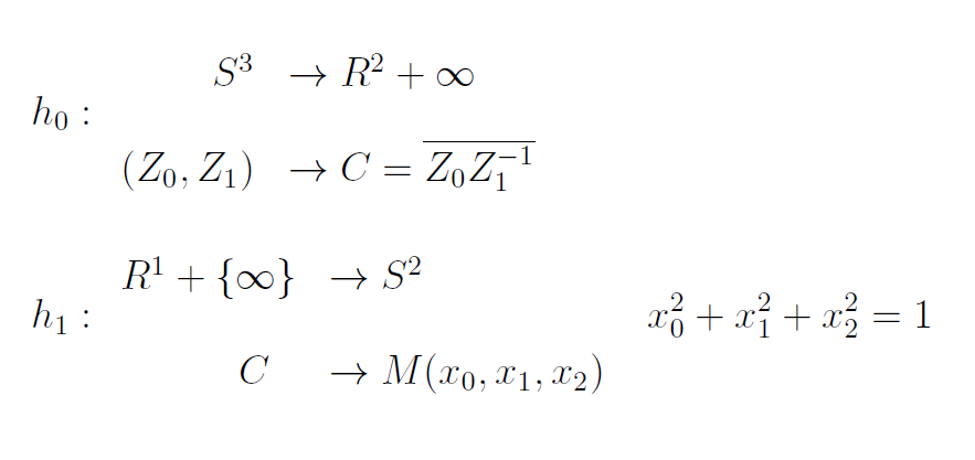 From there, we obtain
\begin{equation}
C=\frac{n_0}{n_1}e^{i(v_0-v_1)}=X_0+X_1 \textbf{i}
\end{equation}
where $\textbf{i}$ is the imaginary number, and (using Euler formula)
\begin{equation}
X_0=\frac{n_0}{n_1}\cos{(v_0-v_1)}, X_1=\frac{n_0}{n_1}\sin{(v_0-v_1)}
\end{equation}
Since (Z_0,Z_1) are points on the sphere, we could write the following equations:
\begin{equation}\label{Stereo}
\begin{split}
u=&\frac{\cos \nu_1}{\sqrt{1+|C|^2}},\\
v=&\frac{\sin \nu_1}{\sqrt{1+|C|^2}},\\
u'=&\frac{X_0\cos \nu_1-X_1 \sin \nu_1}{\sqrt{1+|C|^2}},\\
v'=&\frac{X_0\cos \nu_1+X_1 \sin \nu_1}{\sqrt{1+|C|^2}}.
\end{split}
\end{equation}
Using these parameters, we can use Mathematica to map the coordinates $(u,v,u',v')\in \mathbb{S}^4$ to $(x,y,z)\in \mathbb{R}^3$ using projection maps (see appendix A):
\begin{equation}
\begin{split}
&\pi: S^3\rightarrow \mathbb{R}^3\\
&(Z_0,Z_1)\in \mathbb{C}^2 \longmapsto \pi(Z_0,Z_1)
\end{split}
\end{equation}
From there, we obtain
\begin{equation}
C=\frac{n_0}{n_1}e^{i(v_0-v_1)}=X_0+X_1 \textbf{i}
\end{equation}
where $\textbf{i}$ is the imaginary number, and (using Euler formula)
\begin{equation}
X_0=\frac{n_0}{n_1}\cos{(v_0-v_1)}, X_1=\frac{n_0}{n_1}\sin{(v_0-v_1)}
\end{equation}
Since (Z_0,Z_1) are points on the sphere, we could write the following equations:
\begin{equation}\label{Stereo}
\begin{split}
u=&\frac{\cos \nu_1}{\sqrt{1+|C|^2}},\\
v=&\frac{\sin \nu_1}{\sqrt{1+|C|^2}},\\
u'=&\frac{X_0\cos \nu_1-X_1 \sin \nu_1}{\sqrt{1+|C|^2}},\\
v'=&\frac{X_0\cos \nu_1+X_1 \sin \nu_1}{\sqrt{1+|C|^2}}.
\end{split}
\end{equation}
Using these parameters, we can use Mathematica to map the coordinates $(u,v,u',v')\in \mathbb{S}^4$ to $(x,y,z)\in \mathbb{R}^3$ using projection maps (see appendix A):
\begin{equation}
\begin{split}
&\pi: S^3\rightarrow \mathbb{R}^3\\
&(Z_0,Z_1)\in \mathbb{C}^2 \longmapsto \pi(Z_0,Z_1)
\end{split}
\end{equation}
Stereographic Projections
Now, we define points on $S^1$ as $(x_0,x_1)$ and points on $\mathbb{R}^1$ as $(X_0)$. By the diagram below (observe the triangles $\triangle PRX_0$ and $\triangle OSX_0$), and since \begin{equation} \tan \omega_2=\frac{1}{X_0}=\frac{1-x_1}{x_0}, \end{equation} we yield \begin{equation} X_0=\frac{x_0}{1-x_1}. \end{equation}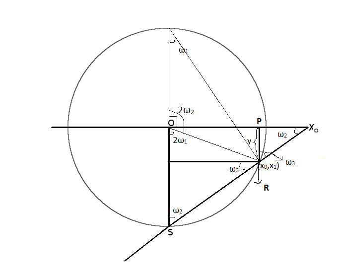
As an analogy to the above construction, we can now define points on $S^3$ as $(x_0,x_1,x_2,x_3)$, then the projection from the south pole $(0,0,0,-1)$ will send the points to the image $(X_0,X_1,X_2)$ by
\begin{equation}\label{CCC} \begin{split} X_0=& \frac{x_0}{1-x_3},\\ X_1=& \frac{x_1}{1-x_3},\\ X_2=& \frac{x_2}{1-x_3}. \end{split} \end{equation} The visualization is done using Mathematica, giving us the following equations: \begin{align} X_0=&\frac{u'}{1-u},\nonumber\\ X_1=&\frac{v'}{1-u},\\ X_2=&\frac{v}{1-u}.\nonumber \end{align} The stereographic projection can also be expressed using polar coordinate system, again by relating triangles $\triangle PRX_0$ and $\triangle OSX_0$, we obtain \begin{equation} X_0=\frac{x_0}{1-y}. \end{equation} But \begin{align} &\tan \omega_1=\frac{x_0}{1+y}, \nonumber\\ &2\omega_2+2\omega_1=180^\circ ,\label{180}\\ &\tan \omega_3=\frac{1-y}{x_0}.------(1) \end{align} Since $\omega_2=90^\circ - \omega_3$, this equation becomes \begin{equation}\label{1=3} \omega_1=\omega_3. \end{equation} Substitute this into equation (1), we obtain \begin{align} \tan \omega_1=\frac{1}{X_0}, \end{align} and the expressions for stereographic projection in polar coordinates: \begin{align} (R,\omega_2)=&\Bigg( \frac{\sin (2\omega_1)}{1-\cos (2\omega_1)},\omega_2\Bigg).\nonumber \end{align}Stereographic projection is a projection from the south pole of $S^3$ to the equatorial three-dimensional hyperplane, the result is a family of nested, coaxial, concentric tori as shown in figure below.
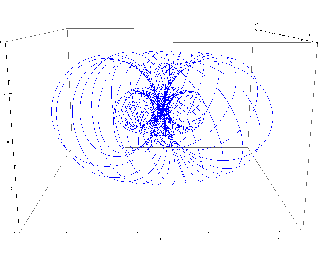 The figure above shows the Stereographic projection of the $S^3$ Hopf fibration, note the nested tori which consist of circles that are linked together, these circles correspond to the points of $(X_0,X_1)$. The infinite line is what we get when we project the south pole (which is our central point of projection) to an extra point at infinity. For $Z_1=0$ we get the circle which sits horizontally on the x-y plane.
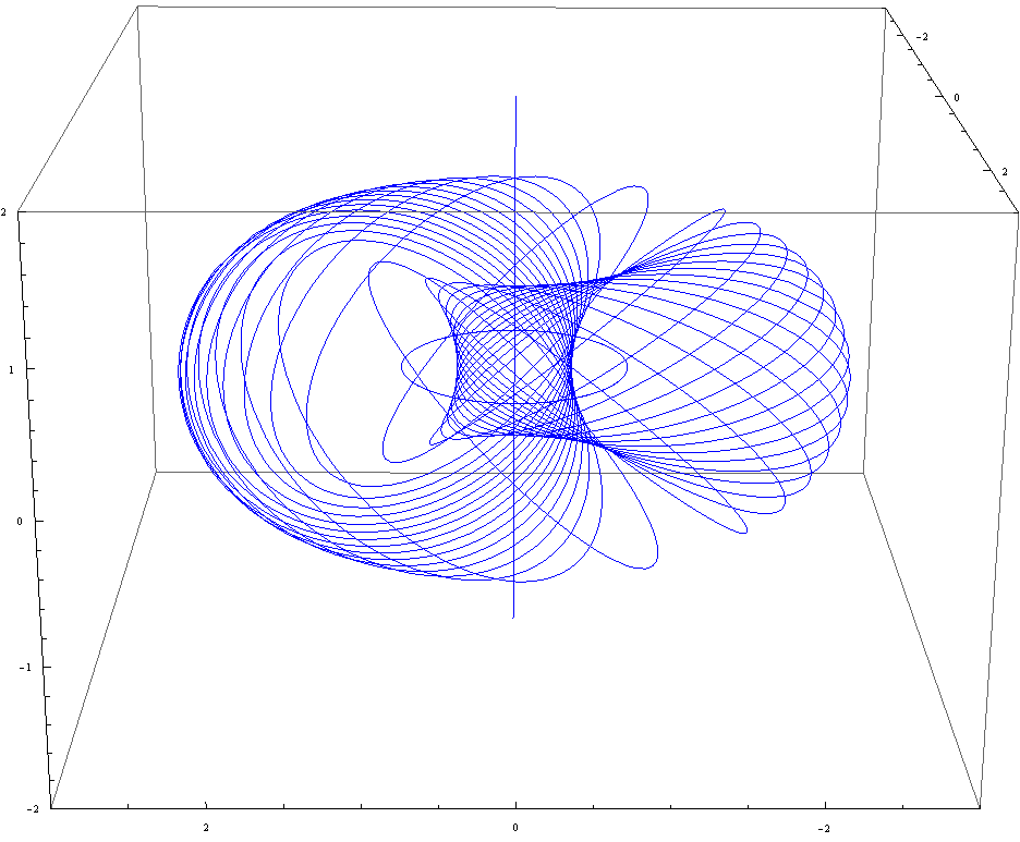 A close-up view of the inner torus along with the disjoint circles.
Properties of Stereographic Projections
Stereographic projection is conformal, i.e. it preserves angles, such that the angle between any two lines on three-sphere must be the same between when these lines are projected to the hyperplane in $\mathbb{R}^3$. Moreover, the coordinates under stereographic projection only has one point not covered, that is, the central point (south pole) where all the great circles that pass through this point will be projected into a line with infinite length as is indicated in figure below.
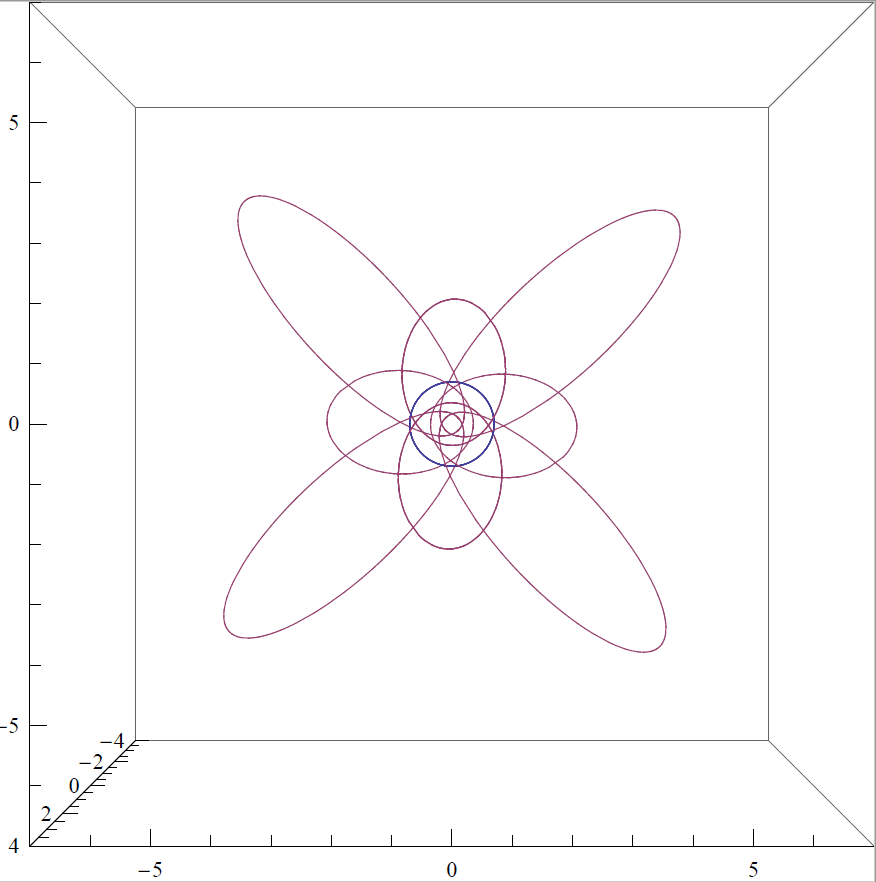 Top view of the stereographic projection with fewer circles, it shows the Villarceau circles which are linked together (in a non-intersecting way as shown by previous figure) to form the nest tori.